Sklearn’s Perceptron

In this chapter I tried out the built in perceptron with sklearn. The code is below

from sklearn import datasets
import numpy as np

iris = datasets.load_iris()
X = iris.data[:, [2, 3]]
y = iris.target

from sklearn.cross_validation import train_test_split
X_train, X_test, y_train, y_test = train_test_split(X, y, test_size=0.3, random_state=0)

from sklearn.preprocessing import StandardScaler
sc = StandardScaler()
sc.fit(X_train)
X_train_std = sc.transform(X_train)
X_test_std = sc.transform(X_test)

from sklearn.linear_model import Perceptron
ppn = Perceptron(n_iter=40, eta0=0.1, random_state=0)
ppn.fit(X_train_std, y_train)
y_pred = ppn.predict(X_test_std)
print('Misclassified samples: %d' % (y_test != y_pred).sum())

from sklearn.metrics import accuracy_score
print('Accuracy: %.2f' % accuracy_score(y_test, y_pred))

from matplotlib.colors import ListedColormap
import matplotlib.pyplot as plt


def plot_decision_regions(X, y, classifier, test_idx=None, resolution=0.02):
    markers = ('s', 'x', 'o', '^', 'v')
    colors = ('red', 'blue', 'lightgreen', 'gray', 'cyan')
    cmap = ListedColormap(colors[:len(np.unique(y))])

    x1_min, x1_max = X[:, 0].min() - 1, X[:, 0].max() + 1
    x2_min, x2_max = X[:, 1].min() - 1, X[:, 1].max() + 1
    xx1, xx2 = np.meshgrid(np.arange(x1_min, x1_max, resolution), np.arange(x2_min, x2_max, resolution))
    Z = classifier.predict(np.array([xx1.ravel(), xx2.ravel()]).T)
    Z = Z.reshape(xx1.shape)
    plt.contourf(xx1, xx2, Z, alpha=0.4, cmap=cmap)
    plt.xlim(xx1.min(), xx1.max())
    plt.ylim(xx2.min(), xx2.max())

    X_test, y_test = X[test_idx, :], y[test_idx]
    for idx, cl in enumerate(np.unique(y)):
        plt.scatter(x=X[y == cl, 0], y=X[y == cl, 1], alpha=0.8, c=cmap(idx), marker=markers[idx], label=cl)

    if test_idx:
        X_test, y_test = X[test_idx, :], y[test_idx]
        plt.scatter(X_test[:, 0], X_test[:, 1], c='black', alpha=1.0, linewidth=1, marker='+', s=55, label='test set')


X_combined_std = np.vstack((X_train_std, X_test_std))
y_combined = np.hstack((y_train, y_test))
plot_decision_regions(X=X_combined_std, y=y_combined, classifier=ppn, test_idx=range(105, 150))
plt.xlabel('petal length [standardized]')
plt.ylabel('petal width [standardized]')
plt.legend(loc='upper left')
plt.show()

When executed it produces a graph showing the decision regions of three flowers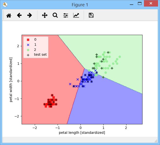

green, red, and blue. It illustrates how the perceptron is not always perfectly efficient, by looking at the misclassified samples.

 

• Uncategorized